Monday, August 06, 2012

It is good to be explicit

Being careful not to repeat the year 1901 mistake, I set the TZ variable before I run R. I have the same set of data that I convert as follows:

dates  <- c("11/11/1900", "01/01/1901", "30/05/1901", "01/01/1902")
values <- c(      1,         2,           0.7,              0.1 )

date1 <- as.Date(    dates, "%d/%m/%Y" )
date2 <- as.POSIXct( dates, "%d/%m/%Y" )

and then plot

plot( date1, values )
plot( date2, values )

To my surprise I end up with the following two graphs.
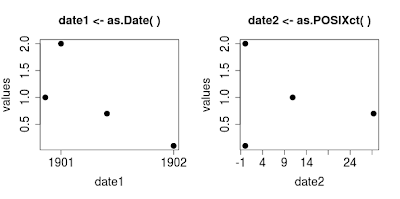
A number of things conspired against me here:

  • positional parameters,
  • default parameters.

Well the main cause is that I did not read the manual and assumed the parameters for as.Date() are similar to those of as.POSIXct(). But ask yourself how many times you used a function without consulting the manual because you thought you knew what the parameters were.

So lets look at the other causes. The help for as.Date() shows the following possible parameters.

as.Date(x, ...)
## S3 method for class 'character'
as.Date(x, format = "", ...)
## S3 method for class 'numeric'
as.Date(x, origin, ...)
## S3 method for class 'POSIXct'
as.Date(x, tz = "UTC", ...)

Depending on the type of object you are trying to convert different parameter lists apply. Lets focus on character objects.

as.Date(x, format = "", ...)

Two parameters are expected:

  • x an object to convert,
  • format a format string that specifies how the dates are formatted.
You can provide values for these parameters positional, that is in the order they are listen, or by name.

An example of the former.

as.Date('1492-11-29', '%Y-%m-%d')
[1] "1492-11-29"

Notice that format also has a default value, "". Which means we do not have to provide it. This indeed works.

as.Date('1492-11-29')
[1] "1492-11-29"

Well sort of. If format equals "" R tries %Y-%m-%d and %Y/%m/%d. It warns when this does not succeed

as.Date('29-Nov-1492')
Error in charToDate(x) : 
  character string is not in a standard unambiguous format

But fails without warning for

as.Date('29-11-1492')
[1] "29-11-14"

29-11-1492 is interpreted as the 29th year, 11-th month and 14-th day. The remaining string "92" not used, but this is not reported.

Default parameters can save time but it is better to be explicit and say what you mean and specify the format of your data, so R does not have to guess, and you won't end up being surprised.

Back to how to provide the values of the parameters. We have seen the positional method, the other one is by name. This would be:

as.Date(x='1492-11-29', format='%Y-%m-%d')
[1] "1492-11-29"

It even works the other way around now.

as.Date(format='%Y/%m/%d', x='1492/11/29')
[1] "1492-11-29"

It is more work to type this, and probably not worth it when you are just using R interactively. But if you are writing a script that is to be reused, this is the best way. It is very explicit, in a good way. You tell R exactly what you mean. In addition you tell your future self what you meant when you wrote it. It help others to understand what you are trying to say. This is good for reproducible research.

Now what went wrong in the original plot? My mistake was to assume that the parameters for as.POSIXct() appear in the same order as the ones for as.Date(). This is not the case however, as can be seen from the help pages.

## S3 method for class 'character'
as.Date(x, format = "", ...)

## S3 method for class 'character'
as.POSIXlt(x, tz = "", format, ...)

Therefore the conversion

date2 <- as.POSIXct( dates, "%d/%m/%Y" )

ended up using "%d/%m/%Y" as the tz parameter. It did not find a value for the format parameter and therefore guessed one (%Y-%m-%d). They day numbers got interpreted as years, and the graph therefore shows the years, 1, 11 and 30. About 2000 years ago instead of the original 100 years given by the data.

I would have avoided the surprising graph had I used named parameters, even without reading the manual.

Conclusion

Be explicit and be beware of implicit defaults in R.

Saturday, July 21, 2012

The magic of the year 1901

The year 1901 is rather magical. Well it is for R provided you run it under Linux. Let me show you why. I have four data points, one from 1900, two from 1901, and one from 1902.

dates  <- c("11/11/1900", "01/01/1901", "30/05/1901", "01/01/1902")
values <- c(      1,         2,           0.7,              0.1 )

I convert them in two different ways; as a Date, and as a POSIXct. For both conversions the same format string is used.

date1 <- as.Date(    dates, format="%d/%m/%Y" )
date2 <- as.POSIXct( dates, format="%d/%m/%Y" )

I plot them like this

plot( date1, values )
plot( date2, values )

Now you try and spot the difference.

Both graphs have the same shape, but different breaks. In the first graph the maximum appears to be in 1901, in the second graph in 1900. This is caused by a bug in the conversion from a string to R POSIXct class.

> as.POSIXct( "1901-01-01", format="%Y-%m-%d" ) 
[1] "1900-12-31 23:59:28 AMT"

Two things are wrong here.

  1. We somehow shifted 32 seconds into the past, (thereby moving from 1901 to 1900, which causes the difference in the two graphs).
  2. We also moved to the CET time zone, where I live, to the Amazonian time zone (AMT).
The conversion works fine for dates in more recent past.

> as.POSIXct("2012-01-01", format="%Y-%m-%d" )
[1] "2012-01-01 CET"

It even works properly for dates before the Unix epoch 1970-01-01.

> as.POSIXct("1957-01-01", format="%Y-%m-%d" )
[1] "1957-01-01 CET"

But around 1940 strange things happen to the timezone, and in december 1901 the 32 second time shift happens.

> as.POSIXct("1940-01-01", format="%Y-%m-%d" )
[1] "1940-01-01 NET"

How to fix this

Be explicit, don't leave R guessing what time zone to use. Set the environment variable TZ to a time zone of your liking before you start R.

$ export TZ=CET
$ R
> as.POSIXct( "1901-01-01", format="%Y-%m-%d" ) 
[1] "1901-01-01 CET"
> as.POSIXct( "1940-01-01", format="%Y-%m-%d" ) 
[1] "1940-01-01 CET"

Thursday, July 19, 2012

Time zones

Say we have some following raw data. It consists of a timestamp and a corresponding value. There is a peak at exactly midnight (00:00:00). Each timestamp is fully specified. It contains a date, a time of day, and a time zone offset indication. In this case +0000, meaning the data is 0 hours away the UTC timezone.

"timestamp","value"
"25-04-2012 22:00:00 +0000",0
"25-04-2012 22:15:00 +0000",0
"25-04-2012 22:30:00 +0000",1
"25-04-2012 22:45:00 +0000",2
"25-04-2012 23:00:00 +0000",5
"25-04-2012 23:15:00 +0000",11
"25-04-2012 23:30:00 +0000",17
"25-04-2012 23:45:00 +0000",19
"26-04-2012 00:00:00 +0000",20
"26-04-2012 00:15:00 +0000",19
"26-04-2012 00:30:00 +0000",17
"26-04-2012 00:45:00 +0000",11
"26-04-2012 01:00:00 +0000",5
"26-04-2012 01:15:00 +0000",2
"26-04-2012 01:30:00 +0000",1
"26-04-2012 01:45:00 +0000",0
"26-04-2012 02:00:00 +0000",0

This data is stored in a file called peak2.dat and we read it as follows:

dataset <- read.csv( file="peak2.dat",as.is=TRUE)

Then we convert the timestamps to POSIXct objects with the aid of strptime. Here we use the %z field to also read the time zone offset:

# Convert timestamps
dataset$timestamp2 <- strptime( format="%d-%m-%Y %H:%M:%S %z",.
                                dataset$timestamp,
                                tz="UTC" )

And use ggplot to make a nice plot of the data. The resulting graph looks something like.

p1 <- ggplot( dataset, aes( timestamp2, value ) ) +.
      geom_point() + scale_x_datetime() 

Something odd happened. The peak that was at 00:00 is now at 02:00 hours.

The reason for this is that the timestamps in the graph are displayed in the timezone of the machine R runs on. In my case this was CET, which is two hours ahead of CET (during summertime).

Notice that if you make the same plot with plot() instead of ggplot() the result is different.

plot( dataset$timestamp2, dataset$value, main="plot()", 
      xlab='timestamp2',
      ylab='value' )

The peak now shows at 00:00 hours instead of 02:00.

So which one is correct. It depends; sometimes you want 02:00, sometimes you want 00:00. Let me give you an example. Say you live in the Germany. You have a collegue living the Iceland. She did some interesting experiment and needs your help analyzing the data. She sends you the data with time stamps with an UTC timezone, the timezone of Iceland (GMT). Also, unlike Germany, Iceland does not have daylight saving.

You analyse the data and make a nice plot with ggplot. You call her an say, "well I see a strange spike 2 o'clock in your data". Then you better tell her it was 2 o'clock your time, or she might go on a wild goose chase trying to figure out what happend during her experiment at 2 o'clock her time. Which depending on the day of the year is 3 o'clock or 4 o'clock your time (depending if you have winter or summer time). In such a case it is much easier to view a graph of the data in the same timezone as where the data is from. Thereby avoiding having to constantly convert back and forth between the timezones.

On the other hand if you have some measuring device that records all timestamps in UTC, and it is located in the same time zone as you, you probably want all time stamps shown in your time zone.

So sometimes you want the data to be shown in your timezone, sometimes in its original timezone. So how can this be acomplished. There are a number of variables that influence how data is shown.

  • The time zone offset of the data (%z field),
  • The parameter tz of the strptime function,
  • The timezone set in your operating system's clock,
  • The environment variable TZ.

The most important variable is the time zone offset. It indicates what the offset is of your timestamp from UTC. It does not indicate the exact timezone, as several timezones can have the same offset from UTC. However if your data includes a time zone offset, use it. With this offset the timestamp defines a single point in time. Without this offset timestamps are ambiguous and the time zone your data is in depends on other variables.

One of these is the tz parameter of the strptime function. It lets you specify the name of a timezone. This parameter does several things. If your timestamp does not include a time zone offset, tz is used to interpret your timestamp.

> x <- strptime( "25-03-2012 02:23:00", 
               format="%d-%m-%Y %H:%M:%S", tz="EST" )
> x
[1] "2012-03-25 02:23:00 EST"

It is also possible to use both time zone offset and tz In this case tz is used when displaying your data.

> x <- strptime( "25-03-2012 02:23:00 +0000", 
                 format="%d-%m-%Y %H:%M:%S %z", tz="EST" )
> x
[1] "2012-03-24 21:23:00 EST"

The value of tz is stored together with the converted timestamp.

> dput(x)
> structure(list(sec = 0, min = 23L, hour = 21L, mday = 24L, mon = 2L, 
    year = 112L, wday = 6L, yday = 83L, isdst = 0L), .Names = c("sec", 
"min", "hour", "mday", "mon", "year", "wday", "yday", "isdst"
), class = c("POSIXlt", "POSIXt"), tzone = c("EST", "EST", "EST"
))

This information is used by some functions that display data.

If you don't specify either time zone offset or tz, R uses the time zone of your OS. But does not store the timezone information.

> x <- strptime( "25-03-2012 02:23:00", format="%d-%m-%Y %H:%M:%S")
> x
[1] "2012-03-25 02:23:00"
> dput(x)
structure(list(sec = 0, min = 23L, hour = 2L, mday = 25L, mon = 2L, 
    year = 112L, wday = 0L, yday = 84L, isdst = 1L), .Names = c("sec", 
"min", "hour", "mday", "mon", "year", "wday", "yday", "isdst"
), class = c("POSIXlt", "POSIXt"))

On Unix like systems you can override this with the environment variable TZ. It puts R temporarily in a different timezone. You would use it as follows:

$ export TZ=EST
$ R 
> x <- strptime( "25-03-2012 02:23:00", format="%d-%m-%Y %H:%M:%S")
> x
[1] "2012-03-25 02:23:00 EST"

The table below shows the effect of these variables on how plot() and ggplot() show the data from the example above. The table shows where the peak of the graph is located for various combinations of the variables. The timezone of the operating system's clock is fixed to CET. The other variables are varied.

time zone offset - UTC
tz strptime - UTC EST - UTC EST
-ggplot 00:00 02:00 07:00 02:00 02:00 02:00
-plot 00:00 00:00 00:00 00:00 00:00 19:00
UTCggplot 00:00 00:00 05:00 00:00 00:00 00:00
UTCplot 00:00 00:00 00:00 00:00 00:00 19:00
CETggplot 00:00 02:00 07:00 02:00 02:00 02:00
CETplot 00:00 00:00 00:00 02:00 00:00 19:00
TZ Plot kind

When we look at the table it is clear that plot and ggplot() behave quite differently. When the timestamps have a timezone indicator, the tz parameter does not have any influence on where ggplot() shows the maximum. For plot() it is the oposite. If no time zone offset is specified, plot() always shows the peak at 00:00.

Conclusion

  • When you make a graph with a time axis be aware in which time zone the breaks on the axis are displayed. Otherwise points of interest might not be where you think they are.
  • Use timestamps with a time zone offset indication,
  • If you want plot() and ggplot() to behave the same, do not use tz but do set TZ.
  • The only(*) way to make ggplot display your data in a different time zone than your OS's, is to set TZ.

(*) ggplot2 used to have a tz parameter for its scale_x_datetime but that seems to be gone in the current release.